A Gentle Introduction to Quantum Mechanics

Quantum Mechanics is often revered for being difficult and unintuitive, and while the results of quantum mechanics deviate from classical mechanics in ways that violate our classical intuition, understanding the mechanics of quantum mechanics is surprisingly accessible.

The goal of this article is to give a gentle introduction to how quantum mechanics work. The goal is not to analyze individual systems in depth, or get bogged down in the often cumbersome details, but rather to get a broad idea of the building blocks of quantum mechanics, and how they interact with each other.

I will try to make the article as accessible as possible, but familiarity with linear algebra, calculus, and some probability theory will be very helpful for the later sections.

In quantum mechanics, we study microscopic systems on the scale of individual or several particles. We can fully describe the state of a quantum system with its wavefunction $\Psi(x,t)$. Think of it as a mathematical object containing all the information we could ever want to know about the system. However, the information we are interested in might not be a very accessible form, so we use special operators $\hat{Q}$ to query the wavefunction to get the information we are interested in.

You might think that, like classical mechanics, the information we might want to query, like position and momentum, is well determined, however, this is not generally the case. The wavefunction is inherently probabilistic, so we have to accept not being able to predict a definitive answer. Indeed this has caused a great many headaches and discussion amongst physicists with Einstein famously saying God "does not play dice".

A surprising thing happens when we query, or measure, a wavefunction with an operator. When we query the wavefunction with an operator, we get a definite result, and the wavefunction changes: it collapses to be in the state associated with the definite result (more on that later). And if we measure the system again with the same operator immediately after, we will always get the same result, so if we want to do repeated measurements, we have to discard the quantum system after each measurement, and prepare a new one in an identical way to before.

If we do repeated measurements on tediously identically prepared systems, we will get a range of values with probabilities determined by $\Psi(x,t)$. But wait! If we measure the position of a particle, and we can get a range of values, where was the particle before we measured it? Surely, it must have been somewhere?

This is the problem that sparked so much discussion. Einstein was a proponent of the realist interpretation where the particle really was at the position we measured it at, and quantum mechanics is incomplete and will one day be superseded by a theory that can predict the position precisely. This is what he meant by his quote.

Many experiments have been performed trying to confirm this, but they haven't been able to find fault with quantum mechanics, so the most widely accepted interpretation today is the orthodox or Copenhagen interpretation championed by Bohr which says that the particle's position really wasn't determined by the universe until the moment it was measured: It wasn't anywhere. The universe didn't know!

The orthodox interpretation is challenging to accept. It's frustrating that we can't fully determine the position before measurement, but I also think there's something beautiful about the extreme lengths the universe goes to in order to be lazy; only determining the outcome of a measurement just in time for the measurement.

Wavefunctions and operators

But what are wavefunctions anyway?

Wavefunctions are vectors living in the Hilbert inner product space which are any function that satisfies $\Psi(x,t)\in\mathcal{H} \Rightarrow \int_{-\infty}^\infty |\Psi(x,t)|^2 dx < \infty$ that is square integrable functions. For a wavefunction to have physical significance, we further require that the integral should be $1$. In practice, we do this by multiplying a constant $A$ so that it fits.

$$P(x\in[a,b])=\int_{a}^b |\Psi(x,t)|^2 dx$$

By convention we write the canonical wavefunction with respect to the position. We could write it with respect to anything we want, and we can, and do, transform the wavefunction between different representations.

Suppose then, we measure the operator $\hat{x}=x$ and get $x\prime$, then $\Psi(x,t)$ collapses to the wavefunction associated with $x\prime$ such that if we measure $\hat{x}$ again immediately after we are guaranteed to get $x\prime$. That is all the mass of the PDF is at $x\prime$ and the integral across the whole space should still be $1$ to make sure the new wavefunction remains a valid PDF. It turns out there's a function that does just that: The Dirac delta function $\delta(x)$ which is $0$ everywhere except at $x=0$ where it's infinite. So $\Psi(x,t)$ collapses to $\delta(x-x\prime)$. It's impossible to measure the position without the wavefunction collapsing into a delta function at the measured position. Measurements are destructive, so we can't recover the original wavefunction from the measurement alone.

However, what if we want to measure something other than the position? And what even is measurable in the first place?

Measurements are done by special operators that query the wavefunction. The operators need to be hermitian so that they have real measurement values (eigenvalues). For an operator $\hat{Q}$ to be hermitian it needs to satisfy

$$\int_{-\infty}^\infty \Psi^* (\hat{Q} \Psi dx) = \int_{-\infty}^\infty (\hat{Q}^* \Psi^*) \Psi dx$$

Or more compactly $\langle \Psi, \hat{Q} \Psi \rangle = \langle \hat{Q}\Psi, \Psi \rangle$ as the integral denotes the inner product of the Hilbert space. Not all operators are hermitian as such not all operators can do physical measurements. The two most important hermitian operators are $\hat{x}=x$ and $\hat{p}=-i\hbar \frac{\partial}{\partial x}$. While $\hat{x}$ looks familiar, $\hat{p}$ looks strange compared to the classical counterpart $p=mv$. You can derive the form of $\hat{p}$ from other parts of quantum mechanics, but at the end of the day, it is a postulate that has been thoroughly verified by experiments. All classical measurables can be written as a function of $\hat{x}, \hat{p}$ . For example, the kinetic energy can be written as

$$T = \frac{1}{2} mv^2 = \frac{\hat{p}^2}{2m}$$

You can verify it classically if you want.

When a hermitian operator $\hat{Q}$ queries, measures, or acts on $\Psi(x,t)$, we write $\hat{Q}\Psi(x,t)$. The possible values of the measurement are the eigenvalues of $\hat{Q}$ that is $q_n \in \mathbb{R}$ such that:

$$\hat{Q}\psi_n = q_n \psi_n$$

The $\psi_n$ are the eigenvectors of $\hat{Q}$. Eigenvectors are special vectors intrinsic to operators that represent the dimensions along which the operator is oriented. When we measure a value $q_n$ with $\hat{Q}$, the wavefunction collapses into the corresponding eigenvector $\psi_n$.

Note: I use eigenvectors, eigenfunctions, and eigenstates as synonyms.

But how do we know the probability of measuring?

Because measurable operators like $\hat{Q}$ are hermitian, their eigenvectors form an orthonormal basis which means any wavefunction can be expressed as a linear combination of the eigenvectors.

$$\Psi = c_1 \psi_1 + c_2 \psi_2 + \cdots = \sum_n^{\infty} c_n \psi_n$$

Then the probability of measuring the eigenvalue $q_n$ associated with the eigenvector $\psi_n$ is $|c_n|^2$. $P(q_n)=|c_n|^2$. Furthermore because the basis is orthonormal, the inner product $\langle \psi_i , \psi_j \rangle$ is $1$ only if $i=j$ and $0$ if $i\neq j$. That is

$$\int_{-\infty}^\infty \psi_i^* \psi_j dx = \begin{cases}1 & : i=j \\0 & : i\neq j \\\end{cases}$$

This is very useful and gives us a way to find the $c_n$ coefficients. If we have an arbitrary wavefunction $\Psi$, and want to find the $n$'th coefficient $c_n$ for the eigenvector expansion of $\Psi$, we can compute $\langle \psi_n , \Psi \rangle$:

$$ \begin{aligned}\langle \psi_n , \Psi \rangle &= \int_{-\infty}^\infty \psi_n^* \Psi dx \\&= \int_{-\infty}^\infty \psi_n^* \sum_i^\infty c_i \psi_i dx \\&= \int_{-\infty}^\infty \sum_i^\infty \psi_n^* c_i \psi_i dx \\&= \sum_i^\infty c_i \int_{-\infty}^\infty \psi_n^* \psi_i dx \end{aligned} $$

But we know from the orthonormality of $\psi_n$ that the integral is $1$ only when $n=i$ and $0$ in all other cases, so we can simplify

$$\langle \psi_n , \Psi \rangle = c_n$$

which is what we wanted to show.

To summarize, measurables are represented by hermitian operators like $\hat{Q}$. The possible outcomes are the eigenvalues of $\hat{Q}$: $q_n$. The probability of measuring a specific value $q_n$ is $|c_n|^2 = |\langle \psi_n, \Psi \rangle | ^2$, and once a specific value is measured, the wavefunction collapses to the associated eigenvector $\psi_n$.

The uncertainty principle

We have already seen that we can't in general predict a definite value for a measurable, but we have also seen that there are special wavefunctions $\psi_n$ for which the probability of measuring a specific value is $100\%$. These are the eigenfunctions of the operator for example $\delta(x-x\prime)$ is an eigenfunction for $\hat{x}$, and a particle described by that wavefunction will always measure the position as $x\prime$.

However, there is an interesting twist to this story. If we have two different operators, we can't, in general, find a wavefunction for which the measurement of both operators can be perfectly predicted. In fact, we are very lucky when we can find shared eigenstates for two different operators letting us fully determine the measurement outcomes of both operators.

For example, if the wavefunction is an eigenfunction for the position, and we attempt to predict the measurement of the momentum operator $\hat{p}$, the variance of the prediction will approach infinity making our prediction equivalent to the ?‍♀️ emoji.

This is another surprising deviation from classical mechanics, and is often summarized as you can't simultaneously measure the position and momentum of a particle. While this gets at the problem, it is not completely true. You can measure the position and momentum simultaneously, but you are limited in the precision of your prediction of your measurement summarized as the variance. Why are you only limited the prediction? Remember when we measure something, we do get precise values, and the system changes to eigenstate associated with that precise value such that rapid subsequent measurements always yield the same value. However, if we measure multiple identical systems the outcome of those measurements will follow the distribution of our prediction.

What happens if our state is not an eigenvector of either the position or the momentum? What is the limit of the combined variance of the two operators? It turns out the lower limit of the product of the variances of two operators $\hat{A},\hat{B}$ is given by

$$\sigma_A^2\sigma_B^2 \geq \left(\frac{1}{2i} \langle \left[ \hat{A}, \hat{B} \right] \rangle \right)^2$$

where $\left[ \hat{A},\hat{B} \right]= \hat{A}\hat{B}-\hat{B}\hat{A}$ is the commutator, and the angle brackets denotes the expectation value. Notice that if $\left[ \hat{A},\hat{B} \right]=0$, then the combined variance needs only be greater than $0$ which is always true, so we can find wavefunctions for which we can fully determine the simultaneous measurement outcomes for both operators. That is the operators share eigenfunctions.

As you might have guessed the commutator for the position and momentum is not $0$. $[\hat{x},\hat{p}]\neq 0 $, so there is a limit to the combined variances. We find

$$\begin{aligned} [\hat{x},\hat{p}]f &= \hat{x}\hat{p}f-\hat{p}\hat{x}f\\ &=x (-i\hbar \frac{\partial}{\partial x})f + i\hbar \frac{\partial}{\partial x} (x f)\\ &= -i\hbar x \frac{\partial f }{\partial x} + i\hbar \left( f + x \frac{\partial f}{\partial x} \right)\\ &= i\hbar f \Rightarrow\\ [\hat{x},\hat{p}] &= i\hbar \end{aligned}$$

Which is perhaps the most important relation in quantum mechanics why we go through pains to derive it. Since the expectation value of $i\hbar$ is $i\hbar$, we find

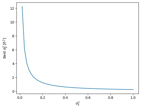
$$\sigma_x^2 \sigma_p^2 = \frac{\hbar^2}{4}$$

How do we interpret this?

We should understand this as a trade-of. The better precision we have in $x$, the worse precision, and the higher the variance in $p$. The relationship is graphed below.

The Schrödinger equation

We have now looked at some of the basic building blocks of quantum mechanics. We have learned that a quantum system is described by a wavefunction, and that we can use operators to query information from the wavefunction. We have also looked at some of the limitations on the precision of the information we get when measuring one or multiple properties, and saw that it deviates from classical mechanics, so can't always know for certain which result we will get.

However, we haven't yet looked at the fundamental problem of mechanics. In mechanics, essentially all problems boil down to given some initial state $\Psi(x,t=0)$, how does the system evolve in time?

In classical Newtonian mechanics, we might know the initial position, the initial velocity, and perhaps an initial acceleration. In quantum mechanics, these values are all summarised in $\Psi(x,t=0)$. To know how the system evolves through time, we also need to know which forces act on the system, and then we can apply Newton's laws to do the time evolution.

In quantum mechanics, we don't use forces, but instead imagine that the particle moves around in a potential $V(x,t)$. We can convert between forces and potential using

$$F(t) = -\frac{d}{dx} V(x,t)$$

You can imagine a potential a bit like biking in rolling hills. If the stretch is flat $\frac{d}{dx} V(x,t)=0$, then there are no forces, and outside friction, and your pedaling, your initial conditions don't change in time. If you're going downhill, you will accelerate towards the bottom - faster if the hill is steeper - and vice versa if you're going up hill.

The reason for this deviation from Newtonian mechanics is that quantum mechanics was first quantized from the Hamilton formulation, so this way of thinking about position and momentum in a potential also applies to classical mechanics.

The analogue to Newton's laws in quantum mechanics is the Schrödinger equation which reads

$$i\hbar \frac{\partial \Psi(x,t)}{\partial t} = -\frac{\hbar^2}{2m} \frac{\partial^2 }{\partial x^2}\Psi(x,t)+V(x,t)\Psi(x,t)$$

We sometimes write this as

$$i\hbar \frac{\partial \Psi(x,t)}{\partial t} = \hat{H} \Psi(x,t)$$

Where $\hat{H}$ is the Hamilton operator. A very important operator which is defined as the total energy; the sum of the kinetic energy $\frac{\hat{p}^2}{2m}$ and the potential energy $V(x,t)$. So the Schrödinger equation says that the derivative of the wavefunction with respect to time is proportional to the Hamilton operator acting on the wavefunction.

In practice, this differential equation is often difficult to solve, and intractable to solve analytically, so approximations and numerical methods are required. However, in the special case that the potential is not time dependent that is $V(x,t)=V(x)$, we can use separation of variables in time and space, and write $\Psi(x,t)=\psi(x)\phi(t)$ which makes the problem of solving the equation much simpler.

It turns out that the time sensitive part $\phi(t)$ has a problem-independent form

$$\phi(t) = e^{-i t E_n / \hbar}$$

You can verify this yourself, or look it up in any introductory book on quantum mechanics. $E_n$ is a real constant. Why we name it $E_n$$ will become obvious in a moment. It's interesting to note that the norm-square of $\phi(t)$ is $1$, so it does not change the overall normalization of the wavefunction. It's just a factor that we can multiply onto our $\psi(x)$ to get the time dependence. In his famous book Griffith calls this the wiggle factor.

The solution to the spatial part is dependent on $V(x)$ which defines the problem. Specifically we get the equation

$$\hat{H} \psi_n = E_n \psi_n$$

You get this equation from separating the variables, and seeing that the time part is constant, but we also see that this is an eigenequation for $\hat{H}$, and we already know that since $\hat{H}$ is a hermitian operator, then the allowed outcomes of measuring $\hat{H}$ are $E_n$. We remember that $\hat{H}$ is defined as the total energy, so it makes sense that it measures the energy motivating the symbol we use.

But where does the $n$ subscript come from? That's a great question, and is one that is best answered by solving a bunch of problems, but for bound problems, that is $E<\max{V}$, the boundary conditions gives rise to the subscript, so there are merely countably infinite allowed energies as opposed to an uncountably infinite number of allowed energies. It's interesting that this is the case, but it's outside the scope of this article to explore it in depth.

Solving a quantum mechanical system for a time-independent potential is finding the eigenvectors and eigenvalues for $\hat{H}$. From that, we have all the information we would ever want about the system, and the rest is just the sprinkles.

As a last note, we have previously seen that $[\hat{H},\hat{Q}]=0$ means that there are shared eigenfunctions for $\hat{H}, \hat{Q}$, but since $\hat{H}$ is a special operator which defines the time evolution, it is also the case that $\hat{Q}$ is conserved through time under the weak assumption that $\hat{Q}$ does not have explicit time dependence. This comes from the generalized Ehrenfest theorem, but we won't go further into that here.

Conclusion

There are a lot more fascinating ways that quantum mechanics breaks our classical intuition such as with quantum tunneling where particles can go through potential barriers greater than their energy; essentially rolling up a hill taller than you have the energy for, and entanglement where two or more particles can be dependent on each other in such a way that it is impossible to describe the system as a system of separate particles, but these have to wait for another time.

We have come a long way. We have seen the nuts and bolts of quantum mechanics, we have explored the probabilistic and uncertain nature of quantum mechanics and the universe, we have outlined how we would solve the fundamental problem of mechanics: time evolution, and we have briefly touched upon symmetries with $[\hat{H}, \hat{Q}]=0$ which is a fascinating topic in itself.

Hopefully now quantum mechanics seems a little less esoteric and unapproachable even if it all seems overwhelming right now.

If you're interested in learning more, I highly recommend reading and doing the problems in David Griffiths and Darrell Schroeter's "Introduction to Quantum Mechanics" which is a phenomenal book used by the majority of university courses around the world.

By Luna Lux Fredenslund