What Is A Neural Network?
Overview and introduction to feed forward neural networks. Forward propagation is discussed in detail, and we see how we might train a network.
In recent years, neural networks have shown great potential across a wide range of industries with access to large quantities of data, and have come to dominate most other machine learning algorithms.
In the following essays, we will analyse how neural networks work, their effectiveness, and how to use them on actual practical problems.
It's assumed that you have basic familiarity with machine learning in general, and have a good grasp on high school level math.
Broad Overview
The overarching goal of neural networks, and machine learning in general, is to find the hypothesis $h(x)$ that best describes an unknown function $f(x)$ on the basis of some, often estimated, values of $f(x)$ for some $x$.
The goal of Machine Learning is to find a model that mimics the true distribution of the training data.
For the sake of simplicity, we will only consider a special type of neural network called a feed forward network in this essay. In later entries, we will also consider more complex architectures.
Once we understand feed forward neural networks, the same principles easily transfers to the more complicated networks such as convolutional, and recurrent neural networks.
A deep feed forward network consists of a series of neurons organized in layers. Each neuron can be thought of as a computational unit that does a simple calculation based on the input it receives.
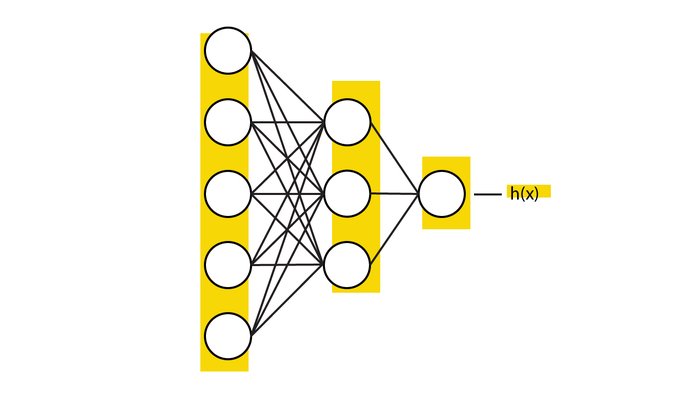
The neurons are connected in such a way that they receive their input from all neurons in the previous layer, and send their output to all the neurons in the next layer as illustrated on the figure above.
The output of the neurons in the final layer is the network's final hypothesis, $h(x)$; what the model thinks the correct answer is.
But what kind of computation do the neurons do, and how exactly do we compute the final hypothesis?
Neural Network Inference
The best way to understand what happens inside a neuron is to show it, which is why I've sketched the calculation done by a single neuron (the yellow one) below:
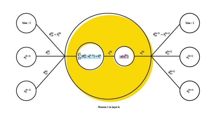
We see here that the neuron computes the sum of the weighted activations of all the neurons in the previous layer, and then add some bias. It then applies a mysterious $g(x)$ function to the result the output of which is the activation of the neuron.
A more general form of the calculation above can be written as:
$$ z_i^{(k)} = \sum_{j=1}^{n^{(k-1)}} \big( \theta_{i,j}^{(k)} \cdot a_j^{(k-1)} \big) + b_i^{(k-1)} $$
$$ a_i^{(k)} = g(z_i^{(k)})$$
Where $a_i^{(k)}$ is a neuron's output, $n^{(k-1)}$ is the number of neurons in the previous layer except the bias neuron whose weighted contribution is denoted $b_i^{(k-1)}$. $g(x)$ is the mysterious activation function; more on that later. $\theta_{i,j}^{(k)}$ is the weight between neuron $j$ in layer $k-1$ and neuron $i$ in layer $k$.
Since the weights are the only thing that seem to change between neurons, you might think that the weights are an important factor in training the network, and you'd be right which we will see later.
In order to compute the network's hypothesis $h(x)$, you need to compute the activations of all the layers until the final layer, $L$, whose neurons outputs $a_i^{(k)}$ together is the network's hypothesis.
But how do we initialize the process? Clearly, we will run out of previous layers eventually.
To initialize the process, we pass in our data, $x$, as the first output of the first layer.
This computation is called forward propagation cleverly named so because you propagate forwards through the network. And you say that mathematicians are bad at naming things.
Matrix Based Neural Networks
While you can do all calculations regarding neural networks without using matrices, it can significantly simplify the notation, and, as we will see later, it is also more time efficient which is why it will be used from now on.
Recall that elements of a matrix, $A$, can be found by: $A_{r,c}$ where $r$ is the row index, and $c$ is the column index. The a matrix then becomes:
$$A=\begin{bmatrix}
a_{(1,1)} & \cdots & a_{(1,c)} \\
\vdots & \ddots & \vdots \\
a_{(r,1)} & \cdots & a_{(r,c)}
\end{bmatrix}$$
The matrix $A$ can be said to have the dimensions: $A\in \mathbb{R}^{r\times c}$ assuming the elements are on the real number line. (Which they are when working with neural networks)
The weights in each layer of the network can be encoded in a matrx $\theta^{(k)}$ each weight can then be accessed by $\theta^{(k)}_{i,j}$. The same can be done for $z^{(k)}$, and $a^{(k)}$.
Matrices have a number of operations defined the most important of which for neural networks being matrix multiplication.
Matrix multiplication is somewhat different from scalar multiplication as it's not commutative.
If $A\in \mathbb{R}^{r\times c}$, and $B\in \mathbb{R}^{a\times b}$, then $AB$ is defined if and only if (iff) $c=a$, and results in a matrix with the dimensions: $AB\in \mathbb{R}^{r\times b}$ which shows why the operation is not commutative. The resulting matrix can be described as:
$$AB=\begin{bmatrix}
a_{(1,1)} & \cdots & a_{(1,b)} \\
\vdots & \ddots & \vdots \\
a_{(r,1)} & \cdots & a_{(r,b)}
\end{bmatrix}$$
Where the elements of matrix $AB$ have the value if we set $c=a=z$:
$$ab_{(i,j)} = \sum_{z=1}^{z} A_{i,z}\cdot B_{z,j}$$
Using matrix multiplication, we can write the big scary expression $z_i^{(k)} = \sum_{j=1}^{n^{(k-1)}} \big( \theta_{i,j}^{(k)} \cdot a_j^{(k-1)} \big)$ as:
$$z^{(k)}=\theta^{(k)}a^{(k-1)}$$
Which is a lot less scary.
Furthermore, we can write almost the entire forward propagation procedure as:
$$\begin{aligned}
z^{(k)} &= \theta^{(k)}a^{(k-1)} \\
a^{(k)} &= g\big( z^{(k)} \big)
\end{aligned}$$
While we are almost there, we haven't yet added the bias term.
To do that in matrix form, we can insert another element in the output, $a^{0}$ with a constant value of $1$. By convention, we will insert the bias term as the first, or the zeroth, element:
$$ a_0^{(k)} := 1 $$
And that's it. That is the complete forward propagation procedure on matrix form.
Feed forward neural networks are essentially just a bunch of matrix multiplications
Activation Functions
Until now, I've teased the mysterious activation function $g(x)$, but I've never said how it is defined.
The purpose of the activation function is to introduce non-linearity into the network which enables it to encode more complex relationships.
We will go into more detail about different activation functions in a later [chapter]() (coming soon), but one historically common activation function is the sigmoid activation which is defined as:
$$ g(x) = \frac{1}{1+e^{-x}} $$
It's not used much today due to numerous problems with it.
If you've taken an introductory course on differential equations, you've probably already encountered it in a more general form as logistic growth.
This function limits the output to be between 0 and 1 which is ideal for binary classification problems.
As activation functions only takes real-valued input, they are applied elementwise when using the matrix-notation.
Toy Example
To solidify our understanding of neural networks, let's consider a very basic toy example.
Suppose we have just two input neurons, a hidden layer with one neuron, and a single output neuron as depicted below:
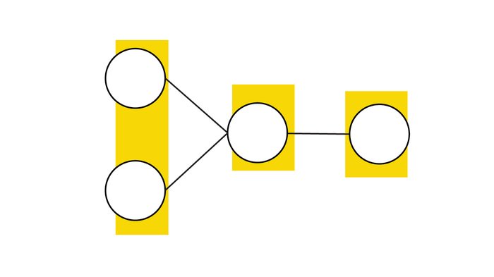
From looking at the illustration, we see that the input vector has two neurons, and two weights. It should be mentioned that I've not drawn the bias unit for any of the layers here.
The hidden neuron has just a single weight associated with it because there's only one output neuron.
How do we find the value of the output neuron?
Since there are two input neurons, we know that the input, $x$, must be:
$$x \in \mathbb{R^{2}}$$
We can find the output value of the first neurons by simply applying the activation function $g()$ on the value.
$$ a_i^{(0)} = g(x_i)$$
We can now calculate the output of the hidden neuron by summing the weighted outputs of the input neurons:
$$ z_1^{(1)} = \sum_{j=1}^{2} \big( \theta_{1,j}^{(1)} a^{(0)}_j \big) + b_1^{(0)}$$
We can now find the output of the hidden neuron like we did with the first layer.
$$ a_1^{(1)} = g(z_1^{(1)})$$
This process can be repeated for the ouput layer as well to find the network's final hypothesis.
You might ask what can this be used for?
One thing that it can be used for is encoding the OR function. Recall the truthtable for OR:
| OR | 1 | 0 |
|---|---|---|
| 1 | True | True |
| 0 | True | False |
If at least one input is 1, then the whole output is True, or 1.
If we let the activation function for the first two layers be:
$$ g(x) = x $$
Which is essentially ignoring the activation, and sigmoid for the output layer, we can use the weights:
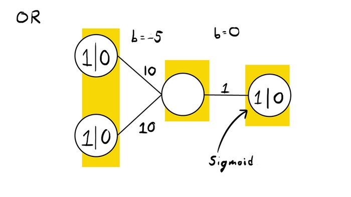
To verify that these weights are correct, we can look at the value of the hidden neuron:
| Hidden Neuron | 1 | 0 |
|---|---|---|
| 1 | 15 | 5 |
| 0 | 5 | -5 |
Between the hidden neuron, and the output neuron, we apply the sigmoid activation function, so we end up with:
| Hypothesis | 1 | 0 |
|---|---|---|
| 1 | $\approx 1 $ | $\approx 1 $ |
| 0 | $\approx 1 $ | $\approx 0 $ |
Which is what we wanted.
In fact, since we could have applied the sigmoid function already on the hidden neuron, it would still work if we removed the hidden unit.
A problem where you have to use a hidden layer is the XOR function. I won't go through what the correct of weights are here, but I encourage you to try figure it out yourself.
Hint: You can use the same architecture as above, but with two hidden neurons.
Until now, we have manually found the values of the weights, but this quickly becomes impractical for large networks, so how do we make the computer automagically find an optimal set of weights?
Training A Neural Network
Neural networks support two modes of operation:
- Inference (Forward propagation)
- Training (Back propagation)
So far, we have only looked at the inference phase which is actually backwards as the training phase comes before the inference phase.
There's too much to cover about the training phase to do it all in detail in just a single essay, so we will only talk broadly about the different components that make up the training phase before going into more detail in later chapters.
In fact, there are multiple ways of training a neural network, but by far the most common method is by using gradient descent with backpropagation which is what we will primarily focus on.
During the training phase you attempt to find a set of weights such that the networks hypothesis $h(x)$, mimics the true distribution $f(x)$. This is the meat of neural networks, and what makes them so effective. We will spend the next couple of chapters how the training process works in depth, but here's a very broad overview.
The training algorithm can be described as follows:
- Start with a bad set of weights
- Iteratively work towards a slightly better set of weights
- Repeat until the weights are good enough
But how do we determine what good weights are?
And how do we know how to update the weights to make them better?
In order to determine how bad the network's current hypothesis is, we use an error function, $E(x,y)$. $E$ should return some distance metric between the label and the hypothesis.
An error function describes how wrong a model's hypothesis is.
The simplest error function, one which you're probably already familiar with, is mean squared error defined as:
$$E(x,y) = \frac{1}{m} \sum_{i=1}^{n} (x_i-y_i)^2$$
Where $m$ is the total number of training examples.
The goal then becomes to find a set of weights that minimizes the value of $E$ across the whole training set.
The weights are updated using an algorithm called gradient descent which iteratively updates each weight in proportion to their influence on the error function.
Neural Networks learn by iteratively changing the weights to minimize an error function
Individual weight's influence on the error function is determined via backpropagation called so because your propagate back through the network starting with the last layer.
We will examine these algorithms closer in the later chapters.
Conclusion
We have looked at how feed forward neural networks are constructed, and how inference works through forward propagation. We have solidified this knowledge by constructing a small example.
Furthermore, have discussed how we might automate the training process.