Creating Your First Machine Learning Classifier with Sklearn
Okay, so you're interested in machine learning. But you don't know where to start, or perhaps you have read some theory, but don't know how to implement what you have learned.
This tutorial will help you break the ice, and walk you through the complete process from importing and analysing a dataset to implementing and training a few different well known classification algorithms and assessing their performance.
I'll be using a minimal amount of discrete mathematics, and aim to express details using intuition, and concrete examples instead of dense mathematical formulas. You can read why here.
At the end of the post you will know how to:
- Import and transform data from a .csv file to use with sklearn
- Inspect the dataset and select relevant features
- Train different classifiers on the data using sklearn
- Analyse the results with the intention of improving your model
We will be classifying flower-species based on their sepal and petal characteristics using the Iris flower dataset which you can download from Kaggle here.
Kaggle, if you haven't heard of it, has a ton of cool open datasets, and is a place where data scientists share their work which can be a valuable resource when learning.
The Iris flower dataset is rather small (consisting of only 150 evenly distributed samples), and is well behaved which makes it ideal for this project.
You might ask why use this admittedly rather boring data-set when there are so many other interesting ones available? The reason is when we're learning about data analysis, using simple, well behaved, data reduces the cognitive load, and makes it easier to debug as we are able to better comprehend the data we are working with.
When learning machine learning the data is less important than how it's analysed.
Importing data
Once we have downloaded the data, the first thing we want to do is to load it in and inspect its structure. For this we will use pandas.
Pandas is a python library that gives us a common interface for data processing called a DataFrame. DataFrames are essentially excel spreadsheets with rows and columns, but without the fancy UI excel offers. Instead, we do all the data manipulation programmatically.
Pandas also have the added benefit of making it super simple to import data as it supports many different formats including excel spreadsheets, csv files, and even HTML documents.
import pandas as pd
import numpy as np
import matplotlib.pyplot as plt
import seaborn as sns

plt.style.use('ggplot') # make plots look better
After having imported the libraries we are going to use, we can now read the datafile using pandas' read_csv() method.
df = pd.read_csv("Iris.csv")
Pandas automatically interprets the first line as column headers. If your dataset doesn't specify the column headers in first line, you can pass the argument header=None to the read_csv() function to interpret the whole document as data. Alternatively, you can also pass a list with the column names as the header parameter.
To confirm that pandas has correctly read the csv file we can call df.head() to display the first five rows.
print (df.head())

# Id SepalLengthCm SepalWidthCm PetalLengthCm PetalWidthCm Species
# 0 1 5.1 3.5 1.4 0.2 Iris-setosa
# 1 2 4.9 3.0 1.4 0.2 Iris-setosa
# 2 3 4.7 3.2 1.3 0.2 Iris-setosa
# 3 4 4.6 3.1 1.5 0.2 Iris-setosa
# 4 5 5.0 3.6 1.4 0.2 Iris-setosa
It's seen that panda has indeed imported the data correctly. Pandas also has a neat function, df.describe() to calculate the descriptive statistics for each column like so:
print (df.describe())

# Id SepalLengthCm SepalWidthCm PetalLengthCm PetalWidthCm
# count 150.000000 150.000000 150.000000 150.000000 150.000000
# mean 75.500000 5.843333 3.054000 3.758667 1.198667
# std 43.445368 0.828066 0.433594 1.764420 0.763161
# min 1.000000 4.300000 2.000000 1.000000 0.100000
# 25% 38.250000 5.100000 2.800000 1.600000 0.300000
# 50% 75.500000 5.800000 3.000000 4.350000 1.300000
# 75% 112.750000 6.400000 3.300000 5.100000 1.800000
# max 150.000000 7.900000 4.400000 6.900000 2.500000
As we now can confirm there are no missing values, we are ready to begin analyzing the data with the intention of selecting the most relevant features.
Feature selection
After having become comfortable with the dataset, it's time to select which features we are going to use for our machine learning model.
You might reasonably ask why do feature selection at all; can't we just throw all the data we have at the model, and let it figure out what's relevant?
To answer this, it's important to understand that features are not the same as information.
Suppose you want to predict a house's price from a set of features. We can ask ourselves if it's really important to know how many lamps, and power outlets there are; is it something people think about when buying a house? Does it add any information, or is it just data for the sake of data?
Adding a lot of features that don't contain any information makes the model needlessly slow, and you risk confusing the model into trying to fit informationless features. Furthermore, having many features increases the risk of your model overfitting (more on that later).
As a rule of thumb, you want the least amount of features that gives you as much information about your data as possible.
It's also possible to combine correlated features such as number of rooms, living area, and number of windows from the example above into higher level principal components, for example size, using combination techniques such as principal component analysis (PCA). Although we won't be using these techniques in this tutorial, you should know that they exist.
One useful way of determining the relevance of features is by visualizing their relationship to other features by plotting them. Below, we plot the relationship between two axis using the plot.scatter() subclass method.
df.plot.scatter(x="SepalLengthCm", y="SepalWidthCm")

plt.show()
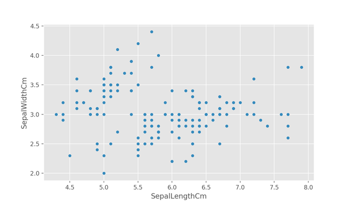
The above figure correctly shows the relationship between the sepal length and the sepal width, however, it's difficult to see if there's any grouping without any indication of the true species of flower a datapoint represents.
Luckily, this is easy to get using seaborn's FacetGrid class where we can use a column to drive the color, or hue, of the scatter points.
sns.FacetGrid(df,
 hue="Species").map(plt.scatter, "SepalLengthCm", "SepalWidthCm").add_legend()

plt.show()
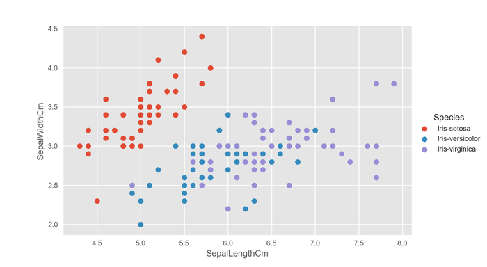
This is much better.
Using the function above with different feature combinations, it's found that PetalLengthCm and PetalWidthCm are clustered together in fairly well defined groups as per the figure below.
Notable is it how the boundary between iris-versicolor and iris-virginca intuitively seems fuzzy. This is something that may cause trouble for some classifiers, and is worth keeping in mind when training.
How did i know how to create those graphs?
I googled it.
When doing machine learning, you will find being able to look up things will be essential. There are endless of things to remember. Spending a lot of time trying to memorize these things is incredibly inefficient. It's more efficient to look things up of which you are unsure, and let your brain automatically remember things you often use.
Being able to quickly look things up is much more valuable than memorizing the entire sklearn documentation.
On the bright side, sklearn is extensibly documented, and well organized making it easy to look up. Sklearn also has a very consistent interface; something you will likely notice throughout the tutorial.
If correlating different features in order to select the best ones sounds like a lot of work, it should be noted that there are automated methods of doing this such as kbest, and recursive feature elimination both of which are available in sklearn.
Preparing data to be trained by a sklearn classifier
Now that we have selected the features we want to use (PetalLengthCm and PetalWidthCm), we need to prepare the data, so we can use it with sklearn.
Currently, all the data is encoded in a DataFrame, but sklearn doesn't work with pandas' DataFrames, so we need to extract the features and labels and convert them into numpy arrays instead.
Separating the labels is quite simple, and can be done in one line using np.asarray().
labels = np.asarray(df.Species)
We could stop now as it's possible to train a classifier using the labels above, however, because the species values' data type is not numeric, but strings, we will run into problems when evaluating the model.
Luckily, sklearn provides a nifty tool that encodes label-strings as numerical representations. It works by going through an array of labels, and encode the first unique label as 0, then the next unique label as 1 and so on.
Using the LabelEncoder follows the standard sklearn interface protocol with which you will soon become familiar.
from sklearn.preprocessing import LabelEncoder
le = LabelEncoder()
le.fit(labels)

# apply encoding to labels
labels = le.transform(labels)
The table below shows labels before and after the data transformation, and was created using df.sample(5).
After Before
139 2 Iris-virginica
87 1 Iris-versicolor
149 2 Iris-virginica
45 0 Iris-setosa
113 2 Iris-virginica
It's seen that each unique string label now has a unique integer associated with it. If we ever want to return to the string labels we can use le.inverse_transform(labels).
Encoding the features follows a similar process.
First, we want to remove all the feature columns that we don't want from the DataFrame. We do that by using the drop() method.
df_selected = df.drop(['SepalLengthCm', 'SepalWidthCm', "Id", "Species"], axis=1)
Now we only have the columns PetalLengthCm and PetalWidthCm left.
Since we want to use more than one column, we can't just simply use np.asarray(). Instead, we can use the to_dict() method together with sklearn's DictVectorizer.
df_features = df_selected.to_dict(orient='records')
The sklearn interface for using the DictVectorizer class is similar to that of the LabelEncoder. One notable difference is the .toarray() method that is used with fit_transform.
from sklearn.feature_extraction import DictVectorizer
vec = DictVectorizer()
features = vec.fit_transform(df_features).toarray()
Now that we have numerical feature and label arrays, there's only one thing left to do which is to split our data up into a training and a test set.
Why have a test set when you can train using all the data? You might ask.
Having a test set helps validating the model, and check for things like overfitting where the model fails to generalize from the training data, and instead just memorizes the answers; this is not ideal if we want it to do well on unknown data. The purpose of the test set is to mimic the unknown data the model will be presented to in the real world. It's therefore very important not to train using the test set.
Sometimes, with algorithms particularly prone to overfitting, you also have a validation set which you want to avoid even looking at because sometimes when optimizing a model, information about the test set may leak from tuning the model parameters (often called hyperparameters) causing it to overfit on the test set as well as the training set.
For this tutorial, however, we will only use a test set and a training set.
Sklearn has a tool that helps dividing up the data into a test and a training set.
from sklearn.model_selection import train_test_split

features_train, features_test, labels_train, labels_test = train_test_split(
 features, labels,
 test_size=0.20, random_state=42)
Interesting here are the test_size, and the random_state parameters. The test size parameter is the numeric fraction of the total dataset which will be reserved for testing. A 80/20 split is often thought to be a good rule of thumb, but may need some adjustment later.
The other notable variable is the random_state. The value of it is not really important as it's just a seed number, but the act of randomizing the data is important.
Why?
The dataset is sorted by type, so if we only train using the first two species, the model won't be useful when testing with a third species which it has never seen before.
If you have never seen something before, it is difficult to correctly classify it.
Choosing a classifier
Now that we have separated the data into test and training sets, we can begin to choose a classifier.
When considering our data a Random Forest classifier stands out as being a good starting point. Random Forests are simple, flexible in that they work well with a wide variety of data, and rarely overfit. They are therefore often a good starting point.
One notable downside to Random Forests is that they are non-deterministic in nature, so they don't necessarily produce the same results every time you train them.
While Random Forests are a good starting point, in practice, you will often use multiple classifiers, and see which ones get good results.
You can limit the guesswork over time by developing a sense for which algorithms generally do well on what problems; of course, doing a first principles analysis from the mathematical expression will help with this as well.
Training the classifier
Now that we chosen a classifier, it's time to implement it.
Implementing a classifier in sklearn follows three steps.
- Import (I usually Google this)
- Initialization (usually self-evident from the import statement)
- Training (or fitting)
In code, it looks like this:
# import
from sklearn.ensemble import RandomForestClassifier

# initialize
clf = RandomForestClassifier()

# train the classifier using the training data
clf.fit(features_train, labels_train)
A trained classifier isn't much use if we don't know how accurate it is.
We can quickly get an idea of how well the model works on the data by using the score() method on the classifier.
# compute accuracy using test data
acc_test = clf.score(features_test, labels_test)

print ("Test Accuracy:", acc_test)
# Test Accuracy: 0.98
98%!
That is not bad for three lines of code. Granted, this wasn't the hardest of problems, but 98% on our first try is still really good.
Note: If you get a slightly different result, you shouldn't worry, it's expeceted with this classifier as it works by generating a random decision trees, and averaging their predictions.
We can also compute the accuracy of the training data, and compare the two to get an idea of how much the model is overfitting. The method is similar to how we computed the test accuracy, only this time we use the training data as for evaluation.
# compute accuracy using training data
acc_train = clf.score(features_train, labels_train)

print ("Train Accuracy:", acc_train)
# Train Accuracy: 0.98
We see that for our training data the accuracy is also 98% which suggests that the model is not overfitting.
But what about entirely new data?
Suppose now we have a found a new, unique, iris flower, and we measure its petal length and width.
Suppose we measured the length to be 5.2cm, and the width as being 0.9cm; how can we figure out which species this is using our newly trained model?
The answer is by using the predict() method as shown below.
flower = [5.2,0.9]
class_code = clf.predict(flower) # [1]
This is great.
We now know the categorical species type. However, the usefulness is limited as it's not easily understandable by humans.
It would be much easier if it would return the species label instead.
Remember the inverse_transform() on the label encoder from before? We can use this to decode the group ID like so:
flower = [5.2,0.9]
class_code = clf.predict(flower) # [1]

decoded_class = le.inverse_transform(class_code)
print (decoded_class) # ['Iris-versicolor']
And so we see that our new flower is of the species Iris versicolor.
Evaluating the results
Even though we can see the test accuracy lies at 98%, it would be interesting to see what kind of mistakes the model makes.
There are two ways a classification model can fail to predict the correct result; false positives, and false negatives.
A false positive is where something is guessed to be true when it's really false.
A false negative is where something is guessed to be false when it's really true.
Since we are not running a binary classifier (one which predict "yes" or "no"), but instead a classifier that guesses which of a series of labels, every mistake will both be a false positive with respect to some labels, and a false negative with respect to others.
In machine learning, we often use precision and recall instead of false positives and false negatives.
Precision attempts to reduce false positives whereas recall attempts to reduce false negatives. They are both a decimal number, or fraction, between 0 and 1 where higher is better.
Formally, precision and recall are calculated like so:
Precision:
$$\text{Precision} = \frac{\text{True Positive}}{\text{True Positive} + \text{False Positive}}$$
Recall:
$$\text{Recall} = \frac{\text{True Positive}}{\text{True Positive} + \text{False Negative}}$$
Sklearn has builtin functions to calculate the precision and recall scores, so we don't have to.
from sklearn.metrics import recall_score, precision_score

precision = precision_score(labels_test, pred, average="weighted")
recall = recall_score(labels_test, pred, average="weighted")

print ("Precision:", precision) # Precision: 0.98125
print ("Recall:", recall) # Recall: 0.98
As seen above, the model has slightly more false negatives than false positives, but is generally evenly split.
Tuning the classifier
Currently, our Random Forests classifier just uses the default parameter values. However, for increased control, we can change some or all of the values.
One interesting paramter is min_samples_split. This parameter denotes the minimum samples required to split the decision tree.
Genereally speaking the lower it is the more detail the model captures, but it also increases the likelyhood of overfitting. Whereas if you give it a high value, you tend to record the trends better while ignoring the little details.
By default it's set to 2.
It doesn't make much sense to lower the value, and the model doesn't seem to be overfitting, however, we can still try to raise the value from 2 to 4.
We can specify classifer parameters when we create the classifier like so:
clf = RandomForestClassifier(
 min_samples_split=4
 )
And that's it.
Train Accuracy: 0.98
Test Accuracy: 1.0
Precision: 1.0
Recall: 1.0
When we retrain the model, we see that the test accuracy has risen to a perfect 100%, but the training accuracy remains at 98% suggesting that there's still more information to extract.
Another parameter we can change is the criterion parameter which denotes how it should measure the quality of a split.
By default it is set to "gini" which measure the impurity, but sklearn also supports entropy which measures the information gain.
We can train the classifier using entropy instead just by setting the parameter like we set min_samples_split.
clf = RandomForestClassifier(
 min_samples_split=4,
 criterion="entropy"
 )
When we retrain the model with the new parameters, nothing changes which suggests maybe the criterion function isn't an important influencer for this type of data/problem.
Train Accuracy: 0.98
Test Accuracy: 1.0
Precision: 1.0
Recall: 1.0
You can read about all the tuning parameters for the RandomForestClassifier on Sklearn's documentation page.
Other classifiers
Another way of improving a model is by changing the algorithm.
Suppose we want to use a support vector machine instead.
Using sklearn's support vector classifier only requires us to change two lines of code; the import, and the initialization.
from sklearn.svm import SVC
clf = SVC()
And that's all.
Running this with just the default settings gives us comparable results to the random forests classifier.
Train Accuracy: 0.95
Test Accuracy: 1.0
Precision: 1.0
Recall: 1.0
We can also use any other classifier supported by sklearn using this method.
Conclusion
Some 3000 words later, first of all congratulations on making it this far. You should celebrate by watching this hamster eating a tiny pizza.
You back? Great!
We have covered everything from reading the data into a pandas dataframe to using relevant features in the data with sklearn to train a classifier, and assessing the model's accuracy to tune the parameters, and if necessary, change the classifier algorithm.
You should now have the tools necessary to investigate unknown datasets, and build simple classification models; even with algorithms with which we are not yet familiar.
Homework
- Optimize the SVM classifier model using the parameters found here.
- Train different classifiers sklearn's documentation may be of use.
- Use the methods discussed in the article to analyse a different dataset for example Kaggle's Titanic Dataset.
For feedback, send your answers to "homework [at] kasperfred.com". Remember to include the title of the blog post in the subject line.
You can access the full source code used in the tutorial here.